
You can have Numbers change the appearance of a cell or its text when the value in the cell meets certain conditions. For example, you can make cells turn red if they contain a negative number. To change the look of a cell based on its cell value, create a conditional highlighting rule.
Select one or more cells.
Click the Cell tab at the top of the sidebar.
If you don’t see a sidebar, or the sidebar doesn’t have a Cell tab, click ![]() .
.
Click Conditional Highlighting, then click Add a Rule.
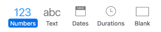
Click a type of rule (for example, if your cell value will be a number, select Numbers), then click a rule.
Scroll to see more options.
Enter values for the rule.
For example, if you selected the rule “date is after,” enter values to specify what date the date in the cell must come after.
Click ![]() to use a cell reference. A cell reference lets you compare the cell’s value to another cell—so, for example, you can highlight a cell when its value is greater than another cell’s. Click a cell to select it, or enter its table address (for example, F1).
to use a cell reference. A cell reference lets you compare the cell’s value to another cell—so, for example, you can highlight a cell when its value is greater than another cell’s. Click a cell to select it, or enter its table address (for example, F1).
After you add a cell reference, you can choose whether a cell reference is relative or absolute. Click the arrow on the token and select Preserve Row or Preserve Column. For more information, go to Calculate values using data in table cells.
Click the pop-up menu and choose a text style, such as Bold or Italic.
You can choose Custom Style to choose your own font color, font weight, and cell fill.
Click Done.
Note: If a cell matches multiple rules, its look changes according to the first rule in the list. To reorder rules, drag the rule name up or down in the order.
After you add a conditional highlighting rule to a cell, you can apply that rule to other cells, too.
Select the cell or cells with the rule you want to delete.
Click the Cell tab at the top of the sidebar on the right.
If you don’t see a sidebar, or the sidebar doesn’t have a Cell tab, click ![]() in the toolbar.
in the toolbar.
Click Show Highlighting Rules, then do one of the following:
Delete all rules for the selected cells: Click ![]() at the bottom of the sidebar, then choose Clear All Rules.
at the bottom of the sidebar, then choose Clear All Rules.
Delete a specific rule: Move the pointer over the rule, then click ![]() in the top-right corner.
in the top-right corner.
Remove a rule from all cells that use it: Click ![]() at the bottom of the sidebar, choose Select Cells with Matching Rules, move your pointer over the rule, then click
at the bottom of the sidebar, choose Select Cells with Matching Rules, move your pointer over the rule, then click ![]() in the top-right corner.
in the top-right corner.