
You can modify a chart’s data references at any time. You can add and remove entire data series, or edit a data series by adding or deleting specific data from it.
While you’re editing a chart’s data references, a small triangle appears on the corner tab of each sheet that contains data used in that chart.
If you can’t edit a chart, it may be locked. Unlock it to make changes.
Tap a chart, then tap Edit References.
Do any of the following:
Remove a data series: Tap the colored dot for the row or column you want to delete, then tap Delete Series.
Add an entire row or column as a data series: Tap its header cell. If the row or column doesn’t have a header cell, drag to select the cells.
Add data from a range of cells: Touch and hold, then drag across the table cells.
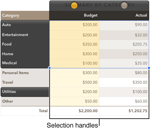
Add or remove data from an existing data series: Tap the colored dot for the row or column, then drag the blue selection handle at the corner of the selection box to include the cells you want.
Tap anywhere on the sheet outside of the chart and table when you’re finished.
Tap a chart, then tap Edit References.
Tap ![]() in the toolbar, then turn on Show Each Series.
in the toolbar, then turn on Show Each Series.
Drag the blue selection handles to include only the cells you want in each series.
Tap Done.
When you add a chart, Numbers defines default data series for it. In most cases, if a table is square or if it’s wider than it is tall, the table rows are the default series. Otherwise, the columns are the default series. You can change whether rows or columns are the data series.
Tap a chart, then tap Edit References.
Tap ![]() , then tap Plot Rows as Series or Plot Columns as Series.
, then tap Plot Rows as Series or Plot Columns as Series.
Tap Done.
When you import a spreadsheet that includes hidden data (data in hidden rows or columns, or data hidden due to data filtering), you can choose to include that hidden data in your charts. By default, hidden data isn’t included.
Tap a chart, tap ![]() , then tap Chart.
, then tap Chart.
Tap Chart Options, then turn on Show Hidden Data.
For more information about how to hide table rows or columns, go to Add and rearrange table rows and columns.