Add conditional highlighting to cells

1. Select a cell or range of cells.

2. In the Cell pane of the Format inspector, click Conditional Highlighting, then click Add a Rule.

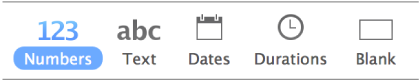
3. Click a type of rule (for example, if your cell value will be a date, select Dates), then click a rule. Scroll to see more options.

   

4. Enter values for the rule.

   For example, if you selected the rule “date is after,” enter values to specify what date the date in the cell must come after.

   Click to use a cell reference. A cell reference lets you compare the cell’s value to another cell—so, for example, you can highlight a cell when its value is greater than another cell’s. Click a cell to select it, or enter its table address (for example, F1).

   After you add a cell reference, you can choose whether a cell reference is relative or absolute. Click the arrow on the token then select Preserve Row or Preserve Column. For more information, go to Calculate values using data in table cells.

5. Choose a style from the pop-up menu.

   You can choose Custom Style to choose your own font color, font weight, and cell fill.

6. Click Done.

The easiest way to add a rule to multiple cells is to select those cells, then add the rule. However, if you already added a rule to a cell and you want to apply that rule to other cells, you can combine highlighting rules.

1. Select the cell with the rule you want to repeat and the cells you want to add the rule to.

2. In the Cell pane of the Format inspector, click Show Highlighting Rules.

3. Click Combine Highlighting Rules.